FDMForward Dynamics Model

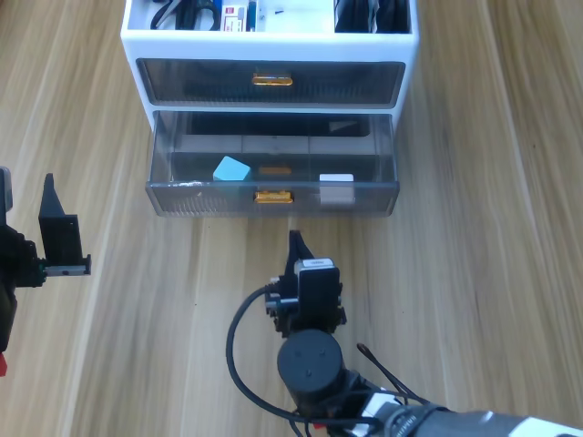
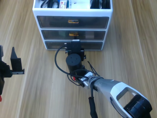
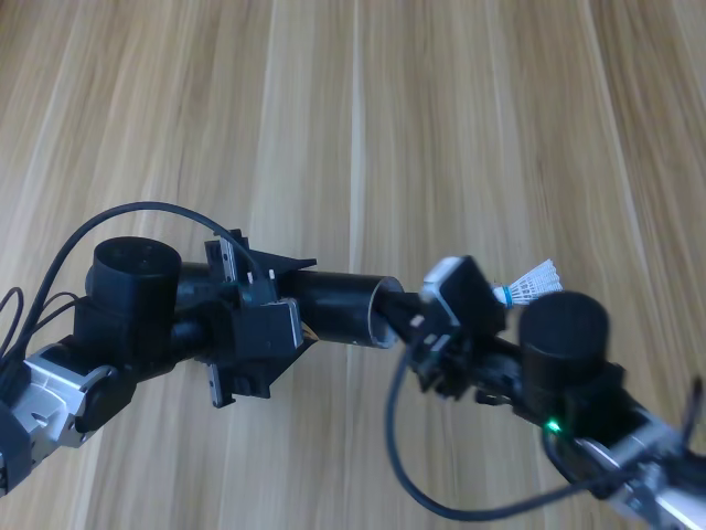
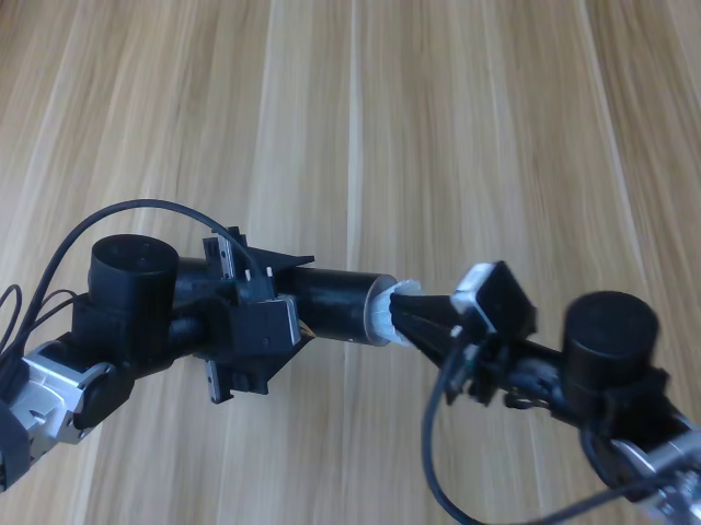
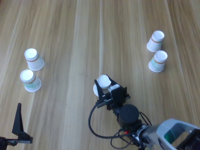
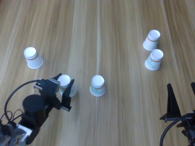
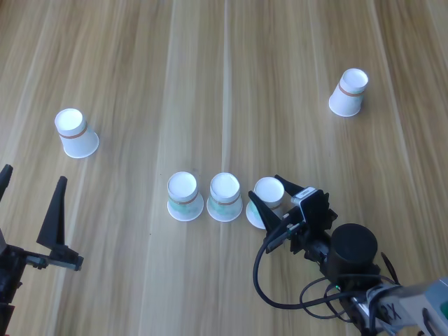
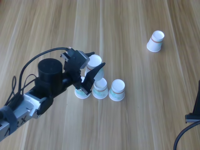
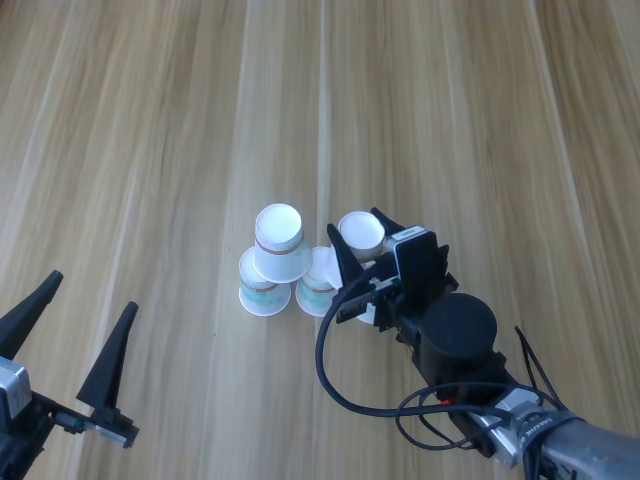
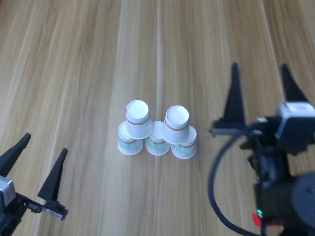
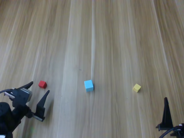
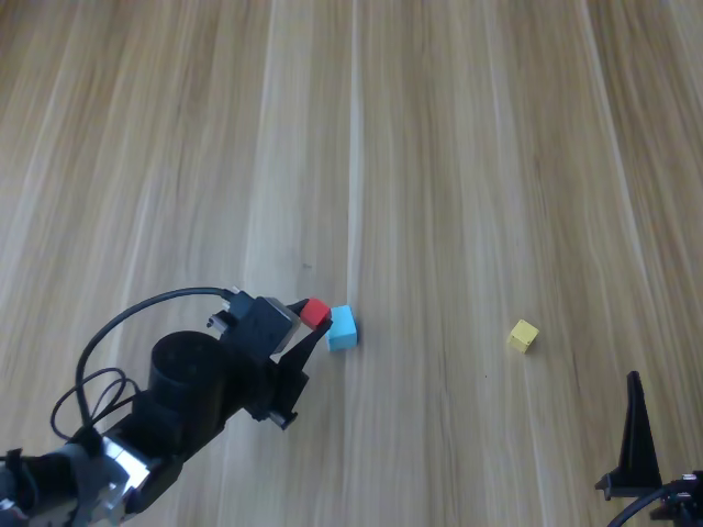
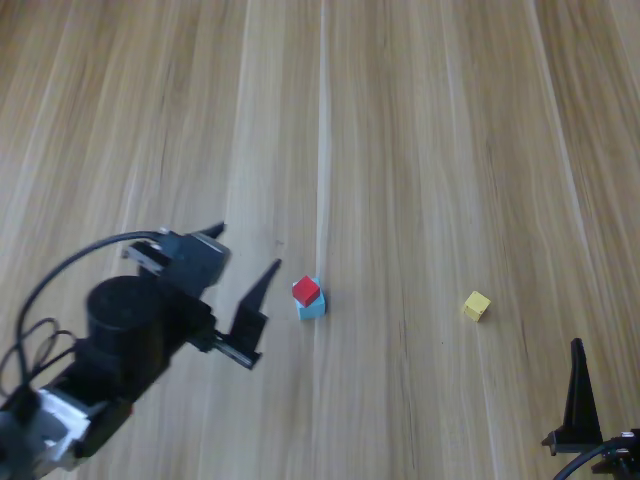
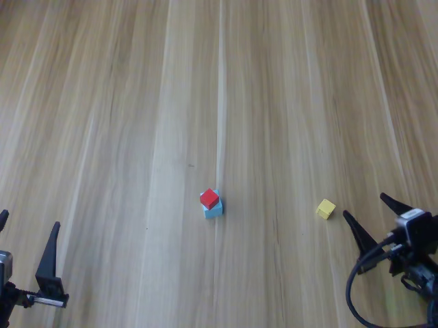
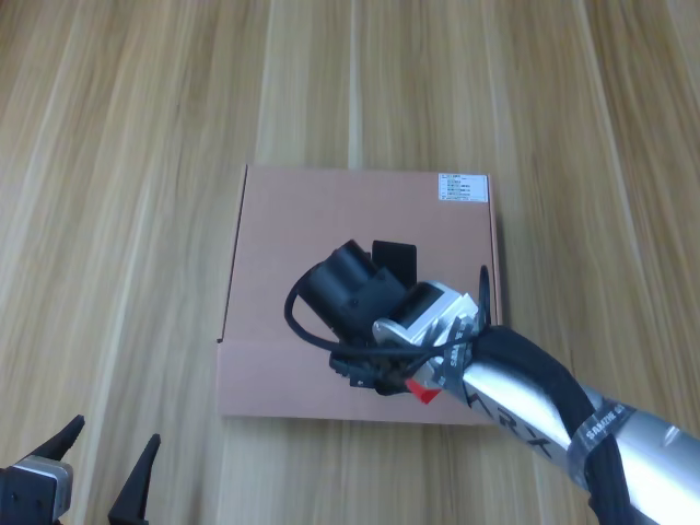
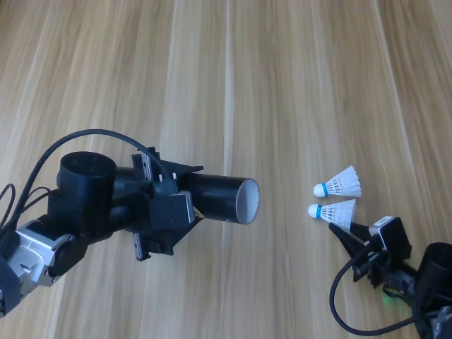
Drawer packing ARX-X5 · 1× speed

From action features to future supervision.Download narrated video

Zipei Ma1,2Junzhe Jiang1Jiahui Zhang1Juntong Zhang2Chun Gu1,2Bozhou Zhang1Jiankang Deng3Xiatian Zhu4Li Zhang1,2

1 Fudan University2 Shanghai Innovation Institute3 Imperial College London4 University of Surrey

What if actions
came before the future?

Future world states are a rich learning signal. FDM uses them to train action features, while keeping predicted futures out of the action path.

Direction of conditioning

(a) VLA

Direct action prediction

VLA: direct action prediction Vision and language enter a vision-language model, which feeds an action expert to predict actions directly. VisionLanguage VLM Vision-language model Action expert Action

(b) WAM

Future-conditioned actions

WAM: future-conditioned actions Vision and language enter a video-generative model. The generated future is an input to the action expert, which then predicts actions. VisionLanguage VGM Video-generative model Future Action expert Action

(c) FDM

Action-to-future learning

FDM: action-to-future learning Vision and language enter a VLM or VGM, then an action expert predicts actions. Context and action features also condition a generation expert to predict the future during training only. Future predictions never feed into the action expert. VisionLanguage VLM / VGM Action expert Action Training only Generation expert Future
Three paradigms, one key difference: the direction of conditioning.Original figure · PDF

VLA

Predict actions from observations and language, without explicit future-state supervision.

Future-conditioned WAM

Generate futures to predict actions. Visual prediction errors can affect the policy.

FDM Our approach

Predict futures from action features. Learn from future states; deploy with action-only inference.

A learning signal.
Not an inference dependency.

Three expert roles, one directional connection. The future-prediction loss flows back through the features that produce actions.

Observation + instruction

Context expert

Understand the scene
and the task.

Action features

Action expert

Predict the robot’s
next actions.

Future-state supervision

Generation expert

Predict the consequences
from action features.

Skipped at inference
Future loss supervises action features

Train jointly with action imitation and future prediction. Asymmetric attention blocks future information from reaching actions, including through context.

Explore the full MoT pipeline
Mixture-of-transformers (MoT)

Scroll horizontally to follow the full pipeline.

FDM mixture-of-transformers pipeline During training, visual and text inputs enter the context expert, and noised actions enter the action expert to produce clean actions. MoT attention injects action features into the generation expert. Predicted and ground-truth futures form the future loss, which backpropagates into action features. During inference, future prediction is skipped. Train / Infer Train: all three experts Infer: context + action Training only Predicted future GT future ℒfuture Clean action Context expert Action expert MoT attention Generation expert Action featuresinjection Input visual Forward flow Backpropagation Future generation skipped Retain the current-observation processing needed by the action expert. Input visual Text Noised action
Action features condition future prediction; the future loss supervises those features.Original figure · PDF

One principle.
Two backbone families.

FDM w/ VLM

A π₀.₅ / PaliGemma policy with direct regression of future-image latents. One future image per camera view, supervised with MSE.

VLM implementation

FDM w/ VGM

A Wan2.2 video backbone with flow matching on future-video latents. Current-observation processing remains in the action path.

VGM implementation

Learning that carries
into the real world.

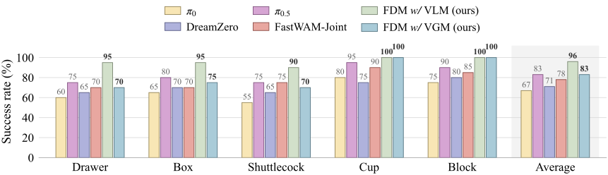
Evaluated in simulation and on a dual-arm ARX-X5 robot. Results below are reported in the paper.

99.4%

LIBERO average success

FDM w/ VLM · four task suites

+13 pp

Real-world success gain

Up to 13 percentage points over compared baselines

1.8×

Faster action inference

FDM w/ VGM vs. FastWAM-Joint · one H100

Five tasks on a real robot

Average · % · higher is better

VLM-based policies

π₀67%

VLA baseline

π₀.₅83%

VLA baseline

FDM w/ VLM96%

Our model

FDM is 13 percentage points above π₀.₅.

VGM-based policies

DreamZero71%

WAM baseline

FastWAM-Joint78%

Future-conditioned WAM

FDM w/ VGM83%

Our model

FDM is 5 percentage points above FastWAM-Joint.

Dual-arm ARX-X5 · 20 trials per method per task · averages across five tasks.

View exact values
Real robot · Figure 5 · all reported values
BackboneMethodSetupDrawer packing (%)Box packing (%)Shuttlecock insertion (%)Cup stacking (%)Block stacking (%)Average (%)
VLMπ₀VLA baseline606555807567
VLMπ₀.₅VLA baseline758075959083
VLMFDM w/ VLMOur model95959010010096
VGMDreamZeroWAM baseline657065758071
VGMFastWAM-JointFuture-conditioned WAM707075908578
VGMFDM w/ VGMOur model70757010010083

Future errors stay
out of the action path.

At perturbation strength α = 1.0, FastWAM-Joint’s action error increases by 4.44% on LIBERO and 5.52% on RoboTwin. FDM’s actions remain unchanged when model parameters, inputs and action-sampling randomness are fixed.
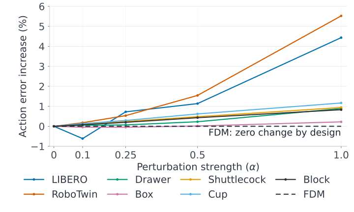
FastWAM-Joint action error generally increases with future perturbation strength across seven settings. FDM is a dashed zero line representing architectural invariance.
Figure 6 · Future-latent perturbationsPaper analysis

The FDM zero line is an architectural property under fixed inputs and randomness, rather than a fitted experimental curve.
Future gradients support
action learning.

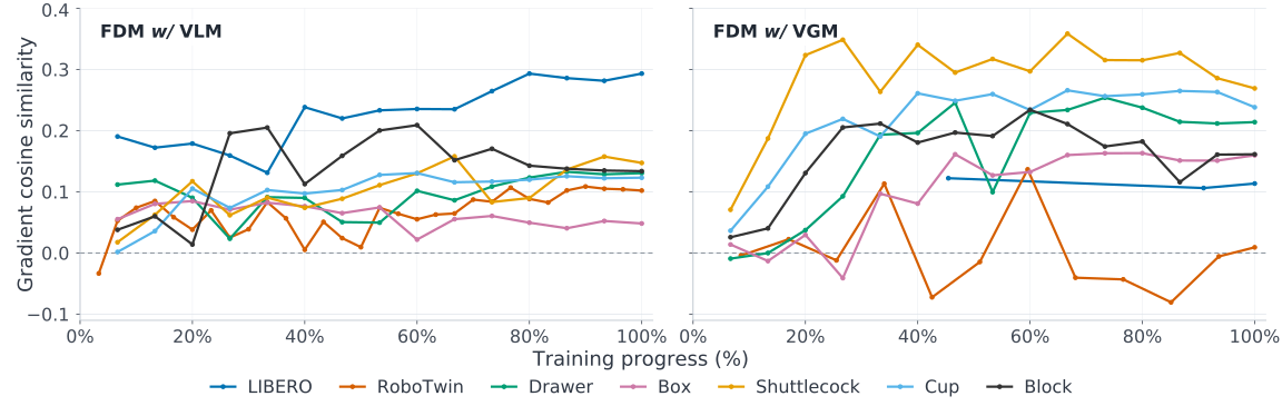
The paper measures cosine similarity between action-imitation gradients and future-loss gradients through the action-feature interface. Alignment is predominantly positive for VLM and positive in most VGM settings after initial fluctuations.

Gradient cosine similarity over training progress for FDM with VLM and VGM, across LIBERO, RoboTwin and five real-robot tasks.
Figure 7 · Shared-context K/V projectionsPaper analysis

The controlled ablations above isolate the behavioral contribution: full FDM improves average success over stop-gradient by 7 points for VLM and 5 points for VGM.

Real-world experiments.

A shared robot setup, five manipulation tasks, and explicit success criteria. Explore how the demonstrations are collected and what each task asks the policy to do.

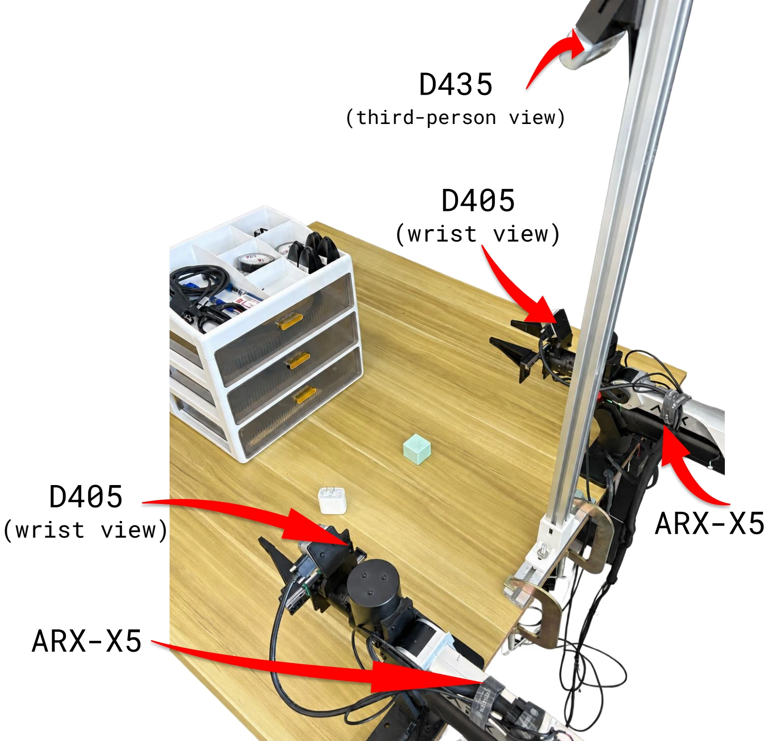
Two ARX-X5 arms face a tabletop. A D405 camera is mounted on each wrist; an overhead D435 captures the workspace from a third-person view.
Figure 9 · Robot and camera layoutOriginal figure · PDF

Experimental setup

Two ARX-X5 arms observe the workspace from three viewpoints. Demonstrations are collected through VR teleoperation.

Robot
Dual-arm ARX-X5
Workspace view
One RealSense D435
Wrist views
Two RealSense D405 cameras, one per arm
Teleoperation
PICO 4 Ultra VR headset
Control
30 Hz · 20-dimensional bimanual actions: position, rotation and gripper commands for each arm

Demonstrations

150 trajectories per task: 147 for training and 3 for offline validation. Object placements vary across demonstrations and evaluation trials.

Evaluation

20 trials per method per task. Human evaluators are blinded to model identity and judge whether the task goal is met. Timeouts and trials judged unable to continue count as failures.

Hardware, collection protocol and task definitions: Appendix D of the paper.

Task details

Inspect six chronological frames from each task in the paper, or jump to the full policy comparisons.

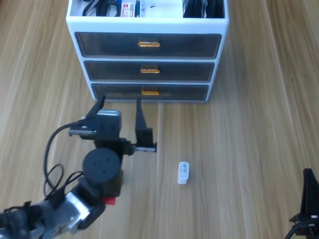
Drawer packing, chronological frame 1 of 6 from Figure 10.
Figure 10 · Frame 1 of 6
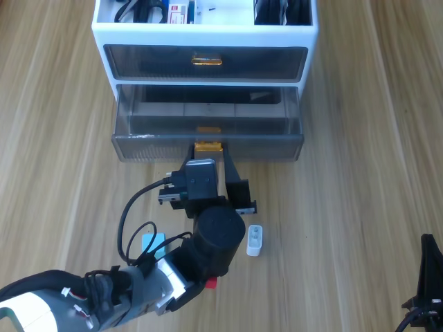
Drawer packing, chronological frame 2 of 6 from Figure 10.
Figure 10 · Frame 2 of 6
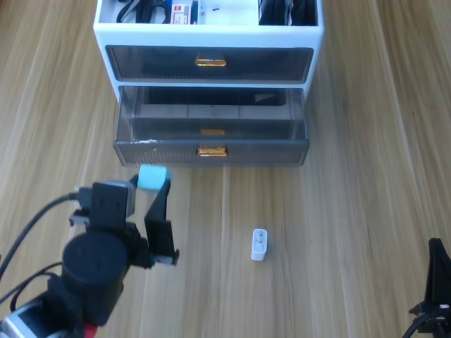
Drawer packing, chronological frame 3 of 6 from Figure 10.
Figure 10 · Frame 3 of 6
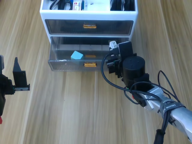
Drawer packing, chronological frame 4 of 6 from Figure 10.
Figure 10 · Frame 4 of 6
Drawer packing, chronological frame 5 of 6 from Figure 10.
Figure 10 · Frame 5 of 6
Drawer packing, chronological frame 6 of 6 from Figure 10.
Figure 10 · Frame 6 of 6

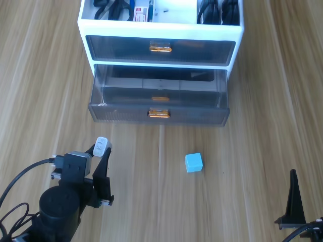
Drawer packing

Put a charger and a block inside an initially closed drawer, then close it again.

  1. Pull the handle to open the drawer.
  2. Pick up and place both objects inside.
  3. Push the drawer fully closed.

Success conditionBoth objects are inside and the drawer is fully closed.

Charger and block positions are randomized; the drawer base shifts slightly.

Box packing and closing, chronological frame 1 of 6 from Figure 11.
Figure 11 · Frame 1 of 6
Box packing and closing, chronological frame 2 of 6 from Figure 11.
Figure 11 · Frame 2 of 6
Box packing and closing, chronological frame 3 of 6 from Figure 11.
Figure 11 · Frame 3 of 6
Box packing and closing, chronological frame 4 of 6 from Figure 11.
Figure 11 · Frame 4 of 6
Box packing and closing, chronological frame 5 of 6 from Figure 11.
Figure 11 · Frame 5 of 6
Box packing and closing, chronological frame 6 of 6 from Figure 11.
Figure 11 · Frame 6 of 6

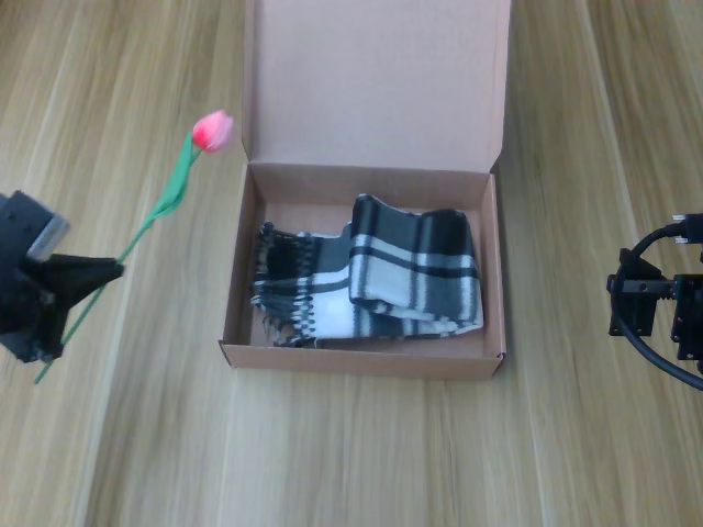
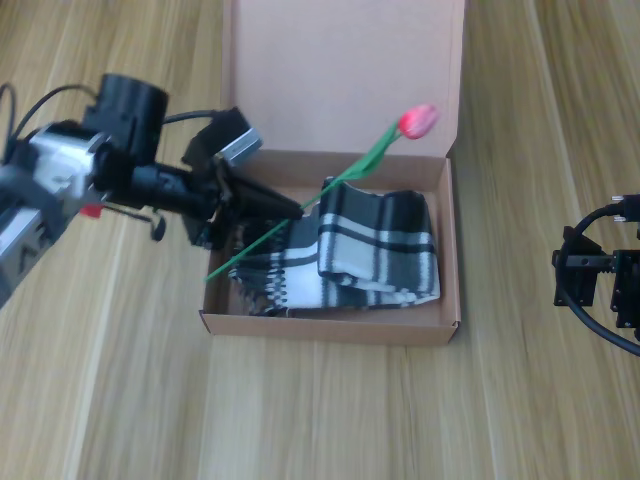
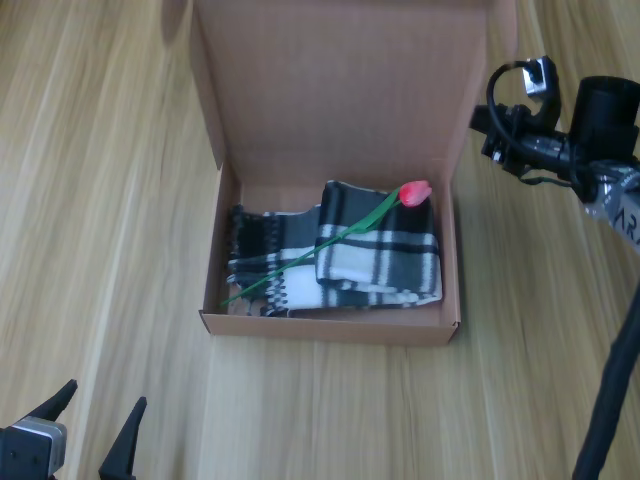
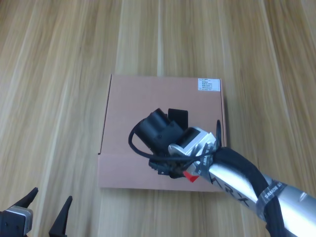
Box packing and closing

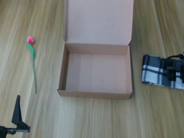
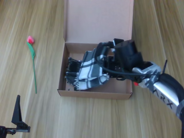
Pack a scarf and a flower into an open box, then close the lid.

  1. Lift the scarf into the box.
  2. Grasp the flower by its stem and place it over the scarf.
  3. Lower the hinged lid without trapping either object.

Success conditionBoth objects are enclosed and the lid is closed.

The positions of the box, scarf and flower vary slightly.

Shuttlecock insertion, chronological frame 1 of 6 from Figure 12.
Figure 12 · Frame 1 of 6
Shuttlecock insertion, chronological frame 2 of 6 from Figure 12.
Figure 12 · Frame 2 of 6
Shuttlecock insertion, chronological frame 3 of 6 from Figure 12.
Figure 12 · Frame 3 of 6
Shuttlecock insertion, chronological frame 4 of 6 from Figure 12.
Figure 12 · Frame 4 of 6
Shuttlecock insertion, chronological frame 5 of 6 from Figure 12.
Figure 12 · Frame 5 of 6
Shuttlecock insertion, chronological frame 6 of 6 from Figure 12.
Figure 12 · Frame 6 of 6

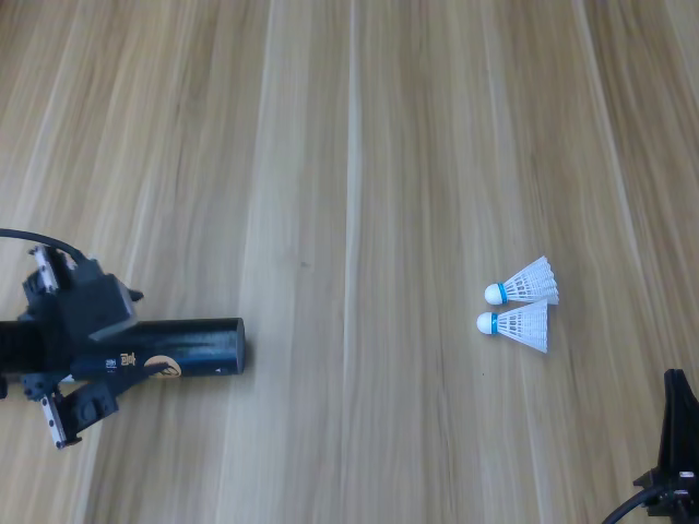
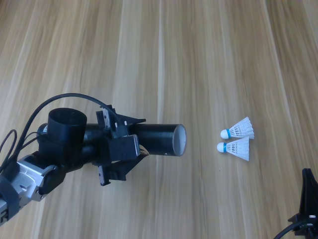
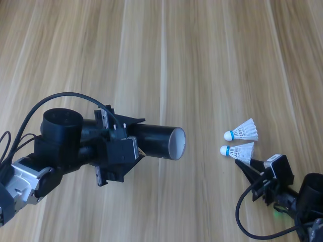
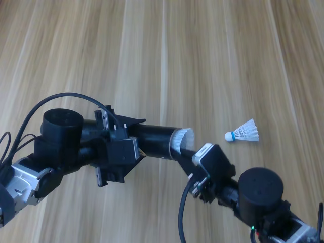
Shuttlecock insertion

Insert two shuttlecocks into a tube using both arms together.

  1. Hold the tube horizontally with one arm.
  2. Align and insert the first shuttlecock with the other arm.
  3. Keep the tube steady and insert the second shuttlecock.

Success conditionBoth shuttlecocks are inside the tube.

The tube shifts slightly; shuttlecock positions and orientations vary.

Paper-cup stacking, chronological frame 1 of 6 from Figure 13.
Figure 13 · Frame 1 of 6
Paper-cup stacking, chronological frame 2 of 6 from Figure 13.
Figure 13 · Frame 2 of 6
Paper-cup stacking, chronological frame 3 of 6 from Figure 13.
Figure 13 · Frame 3 of 6
Paper-cup stacking, chronological frame 4 of 6 from Figure 13.
Figure 13 · Frame 4 of 6
Paper-cup stacking, chronological frame 5 of 6 from Figure 13.
Figure 13 · Frame 5 of 6
Paper-cup stacking, chronological frame 6 of 6 from Figure 13.
Figure 13 · Frame 6 of 6

Paper-cup stacking

Build a two-tier structure: three cups below and two cups above.

  1. Arrange three cups side by side to form the base.
  2. Place the two remaining cups over the gaps in the base.
  3. Withdraw the grippers without disturbing the structure.

Success conditionThe five-cup structure stands freely and stays stable.

Two cups start on the left and three on the right, with randomized positions on each side.

Block stacking, chronological frame 1 of 6 from Figure 14.
Figure 14 · Frame 1 of 6
Block stacking, chronological frame 2 of 6 from Figure 14.
Figure 14 · Frame 2 of 6
Block stacking, chronological frame 3 of 6 from Figure 14.
Figure 14 · Frame 3 of 6
Block stacking, chronological frame 4 of 6 from Figure 14.
Figure 14 · Frame 4 of 6
Block stacking, chronological frame 5 of 6 from Figure 14.
Figure 14 · Frame 5 of 6
Block stacking, chronological frame 6 of 6 from Figure 14.
Figure 14 · Frame 6 of 6

Block stacking

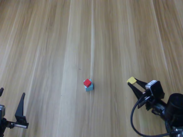
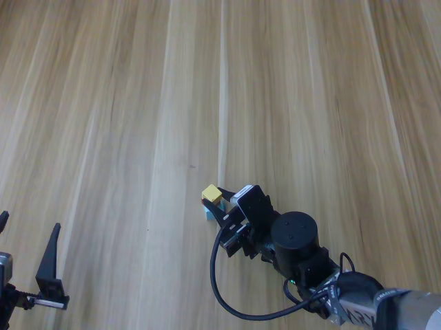
Stack the small red and yellow blocks on the larger blue base.

  1. Pick up the red block and place it on the blue block.
  2. Place the yellow block on top of the red block.
  3. Release and withdraw without disturbing the tower.

Success conditionA stable three-block tower: blue below, red in the middle, yellow above.

Small-block positions are randomized; the blue base shifts slightly.

See the policies in action.

Five manipulation tasks. Four methods. Three camera views. Explore the original real-robot recordings side by side.

Third view on top · Left + right wrist below

Place the objects in the drawer and close it.

Select a task, then play the four recordings together.

Each video combines a 640 × 480 third view above two 320 × 240 wrist views. All views start together; shorter recordings hold their final frame. Displayed duration is the recording length, not model inference latency. Individual clips illustrate behavior; aggregate success uses 20 trials per method per task.

View aggregate real-robot success rates
Paper figure comparing per-task and average success over five real-robot tasks, with 20 trials per method per task. Both FDM variants outperform their corresponding comparison methods on average.
Per-task and average success rates from the paper. Open full-resolution PDF

Five questions from
the experiments.

The main findings, in brief. Each answer links back to the evidence.

Does learning to predict the future improve task success?

It helps across simulation and real-robot tests. On the five real tasks, FDM improves average success from 83% to 96% for the VLM family and from 78% to 83% over FastWAM-Joint for the VGM family. The gains are not universal: on LIBERO, FDM w/ VGM reaches 98.1%, slightly below LingBot-VA’s 98.5%.

Explore task success
Why send the future loss back through action features?

Those gradients make the action features more useful for control. Compared with keeping the same forward connection but stopping its gradients, full FDM gains 7 percentage points for VLM and 5 for VGM on the real tasks.

Compare the ablations
Can a wrong future prediction change the action?

In FDM, actions never read predicted futures, so changing a future prediction leaves actions unchanged when model parameters, inputs and sampling randomness are fixed. FastWAM-Joint depends on those futures: at the strongest tested perturbation, its action error rises by 4.44% on LIBERO and 5.52% on RoboTwin.

See the perturbation analysis
Do future supervision and action imitation work together?

The measured gradients generally point in compatible directions. Their alignment is mostly positive for VLM and becomes positive in most VGM settings after early fluctuations, supporting future prediction as a useful training signal for action learning.

See the gradient analysis
What does FDM cost to train and run?

For VLM, training steps take about 42% longer, while inference stays close to π₀.₅ at about 203 ms per action chunk. For VGM, training cost is nearly unchanged and inference drops from 446.55 to 253.45 ms per chunk, about 1.8× faster than FastWAM-Joint on one H100.

Compare training and inference costs

Condensed from the paper’s experimental questions Q1–Q5. Read the full experiments.

Build on FDM.

Code, training configurations, and evaluation instructions are available in the repository.

View on GitHub

Citation

@misc{ma2026forward,
  title = {Forward Dynamics Models},
  author = {Ma, Zipei and Jiang, Junzhe and
    Zhang, Jiahui and Zhang, Juntong and
    Gu, Chun and Zhang, Bozhou and
    Deng, Jiankang and Zhu, Xiatian and Zhang, Li},
  year = {2026},
  eprint = {2610.13117},
  archivePrefix = {arXiv},
  primaryClass = {cs.RO},
  doi = {10.48550/arXiv.2610.13117},
  url = {https://arxiv.org/abs/2610.13117}
}